
I was quite excited to follow along with Chris French’s series about the limits of skepticism (part 1, part 2 and part 3). During that third part, he fires off an email to one of his collaborators, Julia Mossbridge:
I may well be wrong but I’m having doubts about the probability calculations applied to our results. I know I approved the protocol when you first proposed it and I should have raised this then but I have only now become aware of it. Maybe my concerns are based upon a misunderstanding on my part and you will be able to put my mind at rest. I confess that I do sometimes get in a bit of a pickle when considering probabilities and it’s quite possible I have done so again.
And I relate to that. I was never really taught much about statistics, even at the university level (although signing up for every calculus class that wouldn’t tank my degree might not have helped). Nonetheless, I’ve always had a fascination with how the sausage is made in science, so I’ve spent years teaching myself the fundamentals. I don’t think it’s that hard to pick up; at most it requires some vague memories of how to do algebra, and only if you want to check my work. Even if you instead merely skim and take my word for it, you’ll walk away with a greater understanding of the foundations of modern science.
For better or worse.
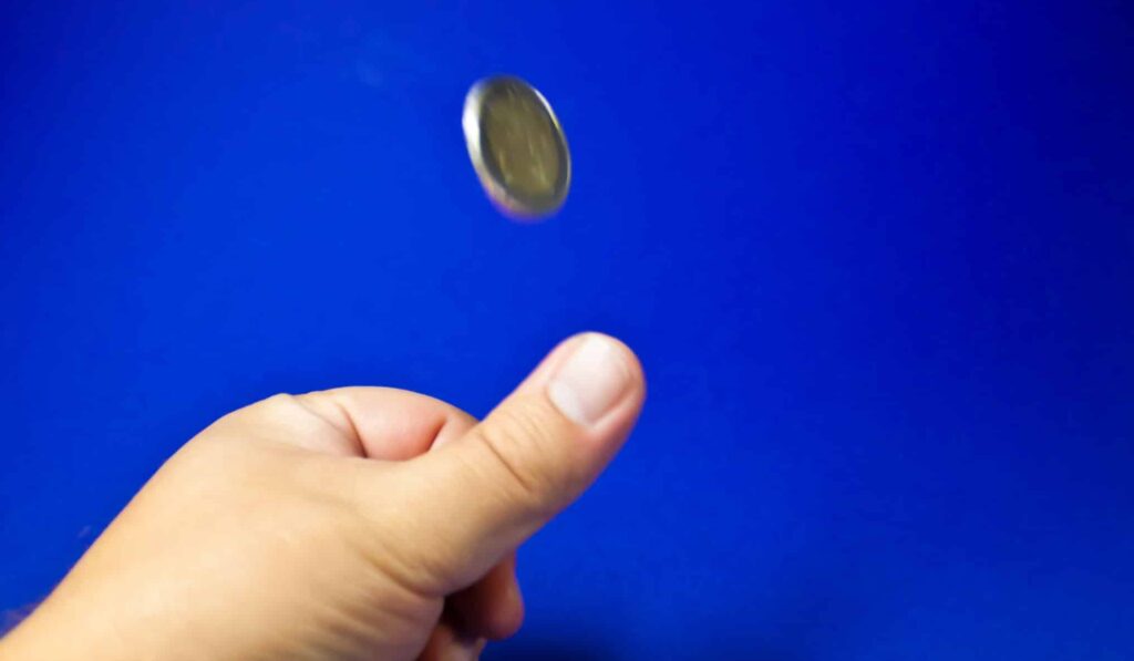
Tossing coins
The workhorse of science is the Bernoulli Process, or what we think we’re doing when we toss a coin. We can toss that coin an arbitrary number of times (the Second Law of Thermodynamics says otherwise), we either get the outcome we want or we don’t (not really), our previous tosses don’t effect this toss (our muscles say otherwise) and, the more we toss that coin, the closer the ratio of total successes to total tosses approaches a fixed constant with a value somewhere between zero and one. How could we prove that convergence?!
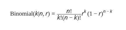
In the magical world of maths, we can just say all of that is true, plus we know what that fixed constant is. We don’t actually know, but we can pretend we do by hiding it behind a variable, r. If that’s our probability of success, our rate of failure must be (1−r). Suppose I toss that coin n times, and it lands heads (which I call a success) k times. You might think the odds of that happening is r multiplied by itself k times, then multiplied by (1−r) a total of (n−k) times, but that’s only true if I got heads k times in a row followed by tails (n−k) times. I could also have tossed some heads, then some tails, then more heads, or any other such combination. We’ve under-counted, but the correction is pretty easy: we multiply by the factorial of n, which is n!=n × (n−1) × ⋯ × 1, then divide by the factorial of k, then divide by the factorial of (n−k).
Congrats, we’ve just reinvented the Binomial distribution! It gives the probability of observing k successes over n trials with a success rate of r. I say “probability” because the Binomial follows the rules of a probability distribution: if we add up the values it produces for all possible values of k (that’s all integers between 0 and n, including both), we get a sum of one.
If Bernoulli Processes are the workhorses, then the Binomial distribution is a prize breed. Prof. French casually name-drops it during one of his articles, and for good reason: Dave Green thought they could predict the future via lucid dreams; French and another person examined 10 dream logs and for each rated how well they matched five candidates, in the end concluding Green got it right three times. That’s k and n, right there!
Removing nuisances
There is a slight problem: what do we do about r? k and n are both integers, which are easy to work with, but r is the sort of thing that ruined Georg Cantor’s life. Let’s set k and n to zero, and see what the Binomial gives us when r is three in ten. Multiplying r by itself zero times seems nonsensical, until dim memories of a math class surface where you were informed that any value raised to the power of zero is one. Calculating the factorial of zero seems equally fanciful (didn’t we stop at one?), but maths boffins have decreed that it equals one as well. So one times one, then corrected by one divided by one and then one again, is… one. The probability of r equalling 3 in 10 is a hundred percent! But we could have substituted any value between zero and one for r, and got the same result.
We need a different type of addition to handle r, and fortunately we have it: integration. I can hear your screams from here, so let me assure you we won’t do any actual calculus around here. Calm yourself down by thinking of a rectangle instead. If that rectangle is one unit high and one unit wide, it has an area of one square unit. If it has a width less than one, then it has an area equal to that width times one.
Notice anything interesting about that rectangle? If I were to randomly pick a number between zero and one, and any number I pick is equally probable to any other I could have picked, the probability of me picking a value between zero and one is 100%. The odds of picking a value between zero and three-tenths is three-tenths, and the odds of picking a value between r and one is (1−r).
We can think of the Binomial distribution with k and n set to zero as a rectangle of height one, and we can think of that rectangle as representing the probability of observing a random number between zero and one. When I plugged an arbitrary value of r into that Binomial distribution, I always get back a value of one; if two outcomes are equally likely to occur, their probabilities must be equal.
Pseudo-probabilities
When we fix k and n and plug r into the Binomial distribution, we get back something that is probability-ish. Under certain conditions it can act like a probability, but if we just call it that we’re likely to forget those conditions. So we we call it a “likelihood”. Hooray for synonyms.
If this “likelihood” is a kind-of-sort-of probability, then it had better sum to one when “added.” Thankfully, the boffins have handed us this gadget:

That’s known as the Beta distribution, and it… hang on, I’m feeling a bit of déjà vu here.
The Beta distribution looks an awful lot like the Binomial distribution, doesn’t it? If we set α to (k+1) and β to (n−k+1), then the bits involving r match up exactly. But does that mean k!=Γ(k+1)? It does! That squiggle is the capital letter Gamma from the Greek alphabet, and the Gamma function is an “all-terrain” factorial; while the original only works for positive integers or zero, the Gamma function handles fractions and complex values with ease (negative integers pop the tyres, alas).
The only difference between the two distributions comes from the numerator, as (k+1) + (n−k+1) = n+2 and thus Γ(n+2) translates into n!(n+1). Or, the Beta’s likelihood is (n+1) times greater than the Binomial’s, when all other values are equal, and that factor compensates for letting r roam free instead of k. We got lucky with the n=0 case earlier, because n+1=1 and thus the Binomial and Beta distributions matched exactly.
But if all values of r are equiprobable when n=0, that implies that before any observations are made our potential Bernoulli Process could converge to any rate. Do you think that if we flip a coin repeatedly, the likelihood of it never landing heads is the same as the likelihood of it landing heads half the time are equal? Surely not! Likewise, you’ll pick the correct image out of five candidates by fluke 1 in 5 times.
Our hypothesis is almost never “each outcome is equally likely.” Even if it is, do you think a million coin tosses will always come up heads exactly half a million times? We are dealing with randomness here, and it’s never that predicable in practice.
Weighing infinities
Just tossing our successes and failures into a Binomial or Beta distribution won’t cut it, we need to find a way to attach a weight to every possible r and do a weighted sum of the probabilities or likelihoods. That was no big deal when we were considering all possible k, as we can count them all, but there are way too many r‘s to count.
Consider the theory that Green would correctly predict 20% of all images, even if their dreams couldn’t predict anything. In that theory’s perfect world, stripped of any randomness, ten trials would result in two successes. A Binomial(2|10,r) distribution can be converted into a Beta(r|3,9) distribution.
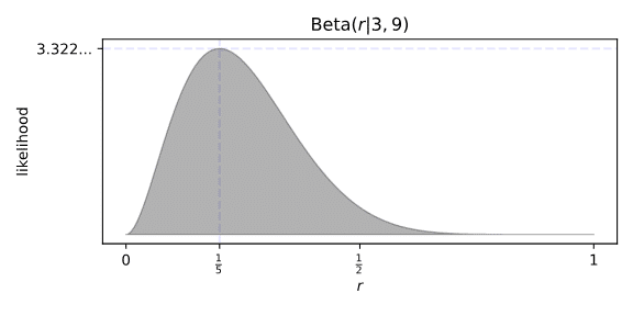
That seems like a pretty good weighting for r. It peaks right at 20%, and covers all possible values. The height of that peak is a bit worrying, but if the Beta distribution is supposed to integrate to one, and it clamps down to zero at both ends plus has a bit of a tail at higher values of r, then the peak must be greater than one. Likelihoods aren’t quite probabilities, after all.
A traditional weighted average is done by adding up each value multiplied by its weight, then dividing by the sum of all weights, and we can skip that last bit if we scale all those weights so they sum to one. Scratch out “addition” and swap in “integration,” and we get
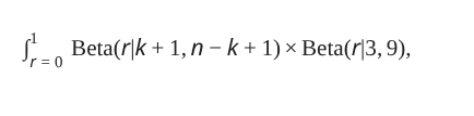
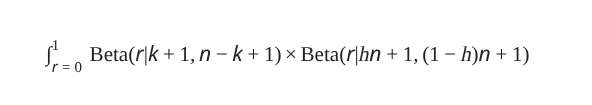
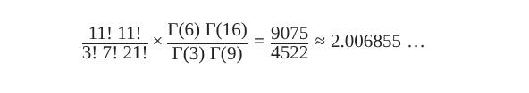
The result would be our average likelihood for the “chance” hypothesis, for k successes over 10 trials. Although, that n looks kind of odd when we’ve baked 20% and n=10 into the math. Let’s instead hide that proposed success rate behind a variable, h, and remove the assumption of ten trials.
I know, I know, the reappearance of that integral symbol has you on edge. Fret not, I wasn’t kidding when I said the Beta distribution was a handy gadget. It lets you solve this integral with basic algebra, no calculus necessary! I’ll leave those who want that challenge to figure it out for themselves, for everyone else I’ll just dish the answer.
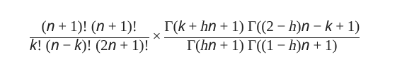
I swapped in factorials where I could, to help organize things, but in practice you’d use nothing but Gamma functions. Whether you think the result is “clean” or not, note that we’ve removed r entirely.
All we have to do now is plug in a few values, and out pops a weighted average likelihood. What are we waiting for? Let’s plug in three successes for Green out of ten trials, with h=210. As per Wolfram Alpha…
Comparing theories
We now have a result! But what does that number mean? With probabilities there was a guaranteed ceiling of 100%. If one possibility had a value of 85%, we knew every other could be no greater than 15% probable. However, likelihoods have no upper limit. Other hypotheses may be more likely or less, we simply cannot tell from a single number.
So let’s look at every number.
The above chart checks every possible h, and returns their weighted average likelihood. The peak is a bit off, but still roughly where we’d expect it. That hill is very smooth, which makes sense: every possible r is assigned a weight by every value of h we pick, and the closer two values of h are the more similar the assigned weights are.
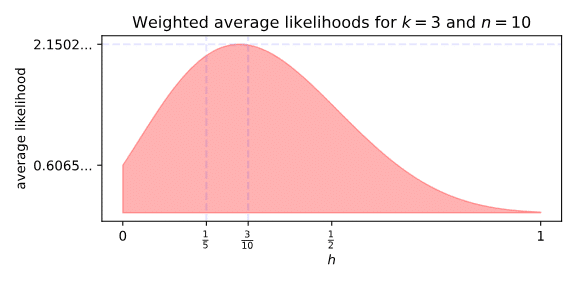
Detour: greater than zero
It doesn’t make sense that the average likelihood of h=0 is anything other than zero, but that very smoothness is the cause. How precise or “peaky” a Beta distribution is depends on the sum of α and β. But since hn+(1−h)n=n for our weighting Beta, how clustered the likelihoods are around h depends only on n.
Intuitively, though, if I’m claiming a value of h equal to one in a million, the likelihoods should be more clustered than if I were instead claiming h is 20%, even if both have the same n. But if that’s true, then how precise is 20% relative to h = 0.2, 0.20, 0.2000, and 0.2000000? If those all have different precision, then r = 0.2000001 has different likelihoods depending on our choice of h. Ugh!
Alternatively, we could stick to our guns. Low values of n cause our weighting Beta to smear across a wide range of r values, overlapping the Beta representing our actual observations. Hence our integral takes uncomfortably large values at the extremes of h. To get comfy, all we need to do is increase n.
Don’t believe me? Let’s detour to my favourite example from this genre. Buried deep in Mossbridge’s citations is this paper:
Bem, Daryl J. “Feeling the future: experimental evidence for anomalous retroactive influences on cognition and affect.” Journal of personality and social psychology 100.3 (2011): 407.
Experiment 2 from that paper involved a computer giving the user the option of picking one of two images. Once the user has picked, the computer randomly decides whether or not the user would get a subliminal “positive” or “negative” image. If the user could predict the future, even slightly, they’d avoid the “negative” image or prefer the “positive” one better than chance.
Still a bit skeptical? Adding a precision term is as simple as calculating s and then swapping hn for shn, (1−h)n for s(1−h)n, and (2−h)n for s(2−h)n.
Comparing theories, for real this time
Oh right, we barely got anywhere on “what does this number mean?” There’s an obvious answer on that chart, the maximum value the average likelihood takes. Since every other value of h is less, we can divide them by it and get back a value safely between zero and one. For an h of 20%, we get a number somewhere around 0.933. The closer to one, the more compatible that theory is with the evidence, so the theory that Green’s performance was a fluke is on solid ground.
It’s an awkward solution, though. Mossbridge’s paper doesn’t just contain the test where French was a judge, it also tasked paid volunteers with evaluating similarity (k=1) and multiple tests where LLMs were judges (k≈3.6). Had I chosen one of those other tests, the maximum likelihood would have been different. It may also have been different had a different set of images been used, or more data points were added, and there’s something unseemly about painting a target around the arrow you’ve shot.
But there’re at least two hypotheses in play on any question. After all, Green is claiming they may be able to predict the future via their dreams. That implies he thinks he succeeded at least once in the past, that he thinks his success rate is better than chance, and he should be able to quantify both theories in some way. We don’t even need a sharp prediction, if we approximate it via a Beta distribution then we can plug that into the maths. A modern computer can evaluate thirty different options before you’ve blinked.
Sadly, Mossbridge’s paper is entirely unhelpful here, even though that information clearly exists:
JM [Mossbridge] agreed that she would be interested if he would be open to attempting to dream pre-cognitively about targets that would be randomly selected after he submitted a dream transcript. DG [Green] agreed, and after a marginally encouraging pilot study, DG suggested bringing open-minded skeptic Chris French (CCF) on board to act as an informed skeptic and another experimental design expert. JM agreed, as did CCF. They then performed another pilot study, which was also encouraging.
I can construct my own “precognitive dreams are real” success rate, with a little help from 13 grad students. They were given a simple task: find a way to flip a coin that biased it towards landing heads. With a few weeks of advance knowledge, and a few minutes of practice, all 13 managed to flip more heads than tails after 300 tosses. And yet coin tosses have a reputation for being fair!
The obvious conclusion is that human beings cannot detect small biases, and thus any person claiming to do better than chance must have produced more than a small bias over chance. Conversely, there wouldn’t be any debate over whether or not anyone can predict the future from dreams if some people had a 99% success rate. With eight and a half billon of us currently running around, and billions more existing in the past, even if only a handful of people could do dream prediction a success rate that high should have been noticed. Since there is a debate, the average success rate must be a small bias over chance.
We’re both pushed up and pulled down towards the probability of a “small bias,” thus that probability is a natural choice for a success rate. The average success rate of those thirteen students was 56.7%, so let’s call that a “small bias” over a fifty-fifty chance.
Betting on theories
20% isn’t 50%, unfortunately, but we can work around that via gambling. Bookies prefer to use “odds” instead of probability, because it’s more intuitive to them. If they quote something as having 4 to 1 odds against, they’re saying they’ll pay out four dollars for every dollar you bet, if that thing happens.
Calculating odds is trivial, the bookie just tallies up wins and losses, then divides the losses by the wins to get the odds against. These fractional odds are very likelihood-ish, but they differ in that they only apply to Bernoulli Processes. That means we can easily translate a Bernoulli Process probability into odds by dividing that probability r by (1−r), and reversing the process by dividing that odds o by (o+1). Ever heard of 50-50 odds? A 50% success rate translated into odds would be 50, divided by 100 minus 50.
We can think of odds as representing the long-term monetary advantage one person has if the probability of success is really 50%. Our mythical bookie offering 4 to 1 odds would wind up with one dollar in their ledger for every four dollars in ours, if they were that far from reality. What probability r would offer a similar advantage over a 20% success rate? We can use ratios to work that out.
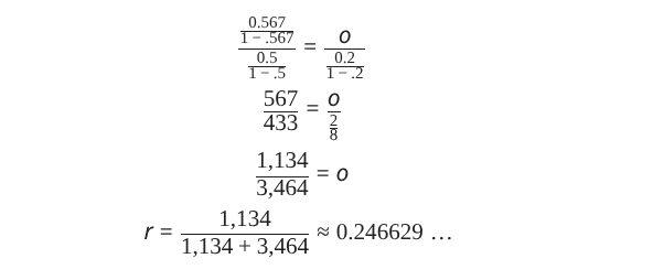
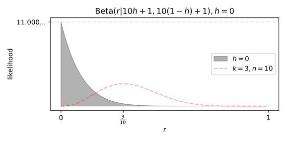
There we go, a ratio of 56.7% to 43.3% odds against 50-50 odds translates to roughly a 24.7% success rate against a 20% success rate. Plugging that into those Gamma functions, we get …
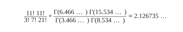
… and the “small bias” hypothesis is more likely than the chance one, given the data. Excellent, Green is vindicated!
But I doubt this has put you in the mood to pop some champagne. The two average likelihoods are nearly identical! We can make your vague feelings more concrete, though, by reversing the process. Likelihoods aren’t tied to Bernoulli Processes, but like probabilities they are proportional: when we say one hypothesis is twice as likely as another, that’s akin to saying we’d place 2 to 1 odds against the other being true.
Suppose I’m on the fence about whether these experiments show Green can predict the future. You’ve walked through all the above maths, though, and know the hypothesis that Green can predict the future is slightly more likely than that he can’t. If I were the clueless bookie from before, how much could you profit off me?

For every dollar I put in, you’d make about $1.06. Or, if you prefer to think in terms of probabilities, your success rate is less than a “small bias”, as we defined it earlier, thus it’s likely I wouldn’t even notice your advantage unless I was keeping careful books.
There is, however, a slight problem: I’m not actually on the fence over whether you can predict the future via dreams. Here’s how the image was selected:
First DG recorded his dream the morning after having had a lucid dream, then sent CCF his transcript. After receiving the transcript, CCF selected a target for the dream at random from a database consisting of 478 pre-pooled online targets. … To select the target from this pool CCF generated a number between 1 and 10 at either Google or Random.org to give the year (1=2006, 10=2016), then two more numbers to give the month and week of the target. … CCF then sent the target URL to DG, who spent between 5 and 120+ minutes reading about the target and viewing any accompanying videos or images.
There’s no way Green could be running a simulation, because he’d somehow have know the exact results returned by Google or random.org, at the exact moment French asked either service to generate random numbers. The latter uses multiple radios scattered across the globe as a source, which is fed through some contraption they haven’t detailed. The former doesn’t say how they generate random numbers, but I bet they just asked French’s browser to do their dirty work.
French may be radiating some mysterious form of thought wave/particles that travel through time, but we’re pretty confident we know all the relevant physics and it can’t be explained by a known force. Time travel is nowhere near practical. The Earth itself orbits the Sun at 30km per second, so any signal would have to not only have to be isolated from billions of others, but to get around the inverse-square law must be focused at a point thousands to millions of kilometres away. I think it’s more likely Green broke into both Google and random.org, sabotaging their random outputs for days at a time in a way nobody noticed… and I don’t think that’s very likely at all!
Still, we should never say something is impossible and, besides, division by zero would break the maths. I’ll instead be exceedingly generous, and put my odds at a million against.

And after taking this evidence in favour of precognition into account, my odds are still roughly a million against predicting the future via dreams. I won’t be popping a cork.
Concluding remarks
I seriously doubt Chris French walked through the above analysis while typing up that email to Mossbridge. But he was doing a similar calculation in his head. The primary difference between the two is that the above is much more rigorous and explicit. I have brushed a few things under the carpet, but if you trust your hammer you don’t really have to know how it’s made. While the maths may have been annoying or opaque to you, it also lays everything out on the table. You can’t critique vague doubts.
Those 10 trials Mossbridge carried out were indeed evidence in favour of the theory that people can predict the future via dreams, it’s just that the amount of evidence they provided was very weak. While that may not be a satisfying conclusion to this story, don’t forget that you’ve now got a hammer in your hand.